A teacher’s guide to creating a department tracker within a reasonable timeframe

Now if you’re anything like me, you have moved from school to school and have always been reliant on that mystical ‘Data Person’ to build your department trackers; a mind-boggling piece of work that has so many different numbers, formulas and ‘don’t touch’ areas that they seem impossible to manage let alone create… unless you have the skillset. Well, hopefully this post will provide you with that skillset.

Honesty alert: I’ll hold my hands up here, the first one I created took me days because I was working away on it like the elves in the shoe shop; late at night or inbetween live teaching. No desk at school was safe from my pencil scribblings as I googled, applied and googled again the formulas I required to build my masterpiece.

Without further adieu, here we go…

Trick 1

Figure out the data you need to produce and track, and which parts of that you need to protect (we all know that one member of the department who will always overwrite something important so that it is lost forever).

In my case, it is the headlines and the grade boundaries.

Set them up in a sperate sheet and then lock that sheet down:

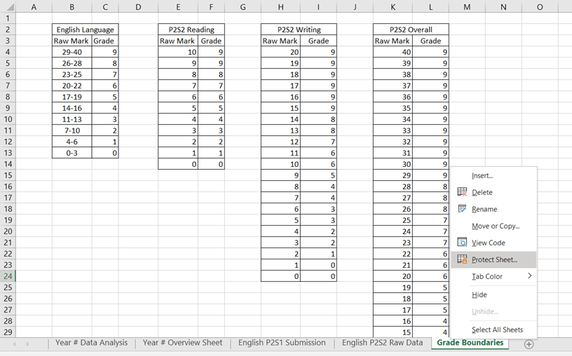
Simply right-click on the sheet you wish to protect, click protect sheet and you will be asked to enter a password, and then to repeat said password:

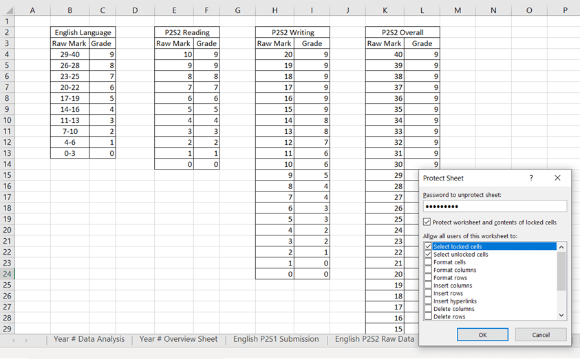
You don’t need to mess around ticking different boxes, unless you want to, by leaving it as it is it will stop anyone from editing the sheet unless they have the ‘golden ticket’.

The only downside to this little trick is that you have to retype the password every time, like new – but that’s just the laziness in me talking.

Trick 1.5

This one didn’t quite deserve a number of it’s own as it’s of a similar nature to Trick 1. This one simply hides the sheet from others views -great if you are using it as a VLookup sheet (I’ll come to that later)

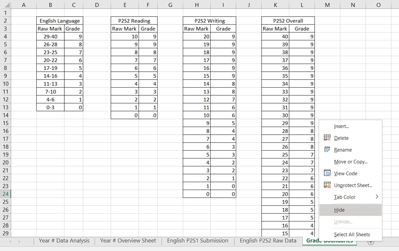
Simply right-click and select hide and POOF it’s gone from view. To unhide it simply right-click on any of the other headers and choose ‘Unhide..’

Trick 2

Okay, so let’s talk about ‘Paste Special’

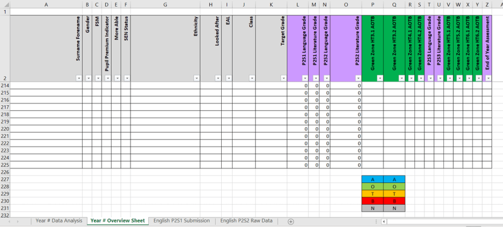
This is where you want something from one sheet to appear on another and update itself automatically. For example, raw data or grades from an assessment point to appear on the Overview sheet, so it is all in one place:

What I want to happen here is for the data from column T to appear on the ‘Year # Overview Sheet’ so that I can see all the information in one place without having to skip back and forth between the sheets.

So what I do here is select the cells I want to copy (in this case T3 onwards – I don’t want to copy all of the headers across) and then on the sheet I want to see the data on I simply ‘Paste Special’ it across:

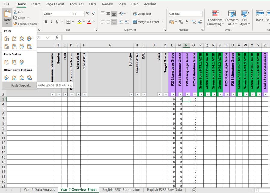
From the arrow underneath Paste button I will be given the option to Paste Special or alternatively press Ctrl+Alt+V for the same outcome. Once I click this I will be given this delightful little option box:

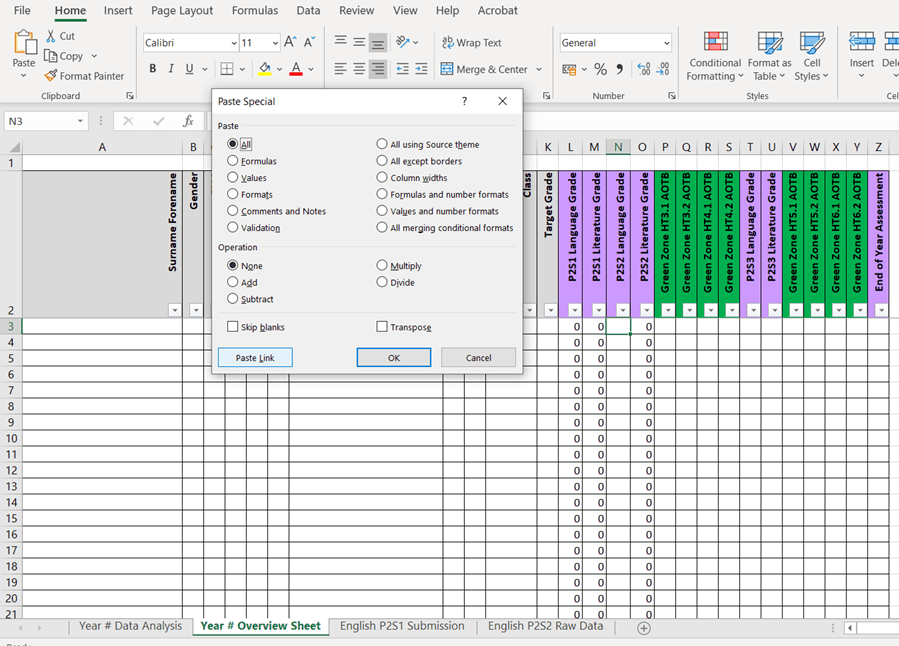
All I need to do now is click ‘Paste Link’ on the bottom left… and vá lá – my selected data has moved across:

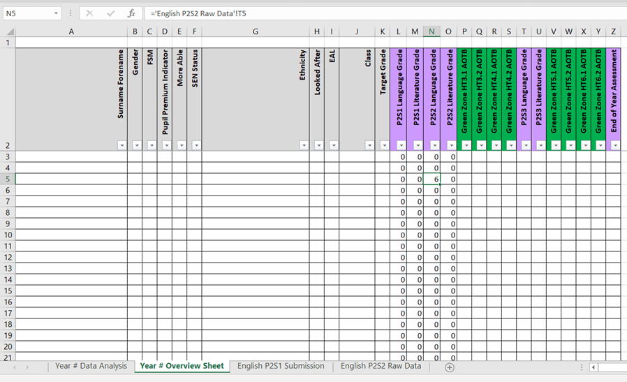
Notice how my Formula Bar now reads ‘=’English P2S2 Raw Data’!T5 which is the name of the sheet and cell I have copied the data from.

Trick 3

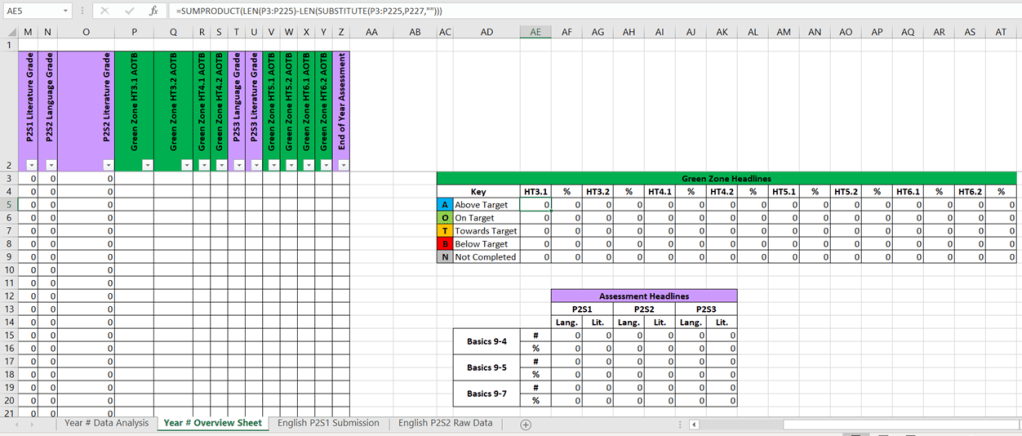
Let’s talk about the Data Analysis sheet – THE BIG ONE.

A little more complicated at first, but once you get the hang of it, it’s as simple as pie. So for this one, I first needed to know what data I wanted to display for my Headlines (it took a few different versions for me to be happy with the final outcome).

For my tracker, I wanted to be able to monitor each of the data drops (P2S on the sheet) in terms of the Headlines I would expect to be questioned on by SLT (not including PP and SEND analysis), which landed me with the Basics 9-4, 9-5 and 9-7.

In an attempt to keep this as simple as possible I will talk about ‘Assessment Headline’ table first, to do this follow me over to the ‘Overview’ sheet:

Step One: The Overview Sheet, Putting the Data in the Right Place

Knowing that I will always have to have quantative data at my finger tips I knew I needed a breakdown of how many students achieved each grade.

As you can see below, I created a ‘Grade Range’ table for each of the data drops with a separate row for each of the grades. This sits directly underneath the main body of the sheet so I can easily hide them later:

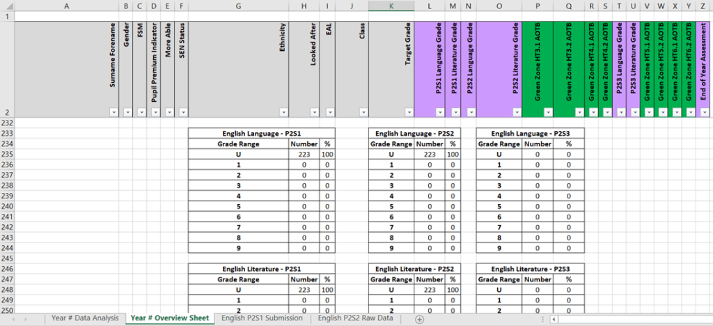
Now in order to drag the data from the information above (each individual students’ data), I entered the ‘COUNTIF’ formula into each cell under the ‘Number’ section in the table; for the U row I entered the follwing:

=COUNTIF (L3:L255,0)

The numbers and letters that come before the comma are for you to edit, these are the cells with the students grades in them in the main body of the sheet. The ‘0’ tells the formula to look for any student who recieved a 0 aka a U (you have to use numbers because for some reason Excel hates letters). For the other cells you would just change the 0 to a 1, 2, 3 etc. depending on the grade you are looking for.

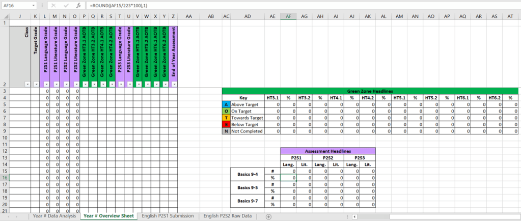
Now, I still want the percentages too. This one baffled me for a while because I wanted a nice round number – no decimals. So for this one I entered the following formula:

=ROUND((H235/223*100),1)

In this case, the letter (H) is the column of the ‘Number’ section (how many kids got that particular grade) and the (235) is the row that contains the information that I want to make into a percentage. The ‘/’ represents divide, and the number that follows it is how many students I have on the sheet (223 in that year group) the ‘*’ represents multiple and then by 100 to get my percentage. The 1 remains the same because I am telling the formula that I want to round to the nearest 1.

Once I’ve created these tables, I simply highlight and right-click on the rows I don’t want the team seeing (as it would just complicate matters) and select hide and POOF they’ve now disappeared from view and hopefully from tampering.

Step Two: The Overview Sheet, Data Sourcing

Now that the unnecessarily complicated I need to create the table I want to see on the ‘Data Analysis’ sheet on the ‘Overview’ sheet (columns AC-AT):

I figured how I wanted it to look – the pretty bit – and then I focused on the bits of data I needed to source. This is where the ‘Grade Range’ tables come in handy. I promise that this step is much more simpler than the previous one…

In the ‘P2S1, Lang. #’ cell I simply typed the following formula in:

=SUM(H239:H244)

The number and letters are the location of the information I need for this cell, i.e. the number of students who achieved a grade 4 or above in P2S1 – this information is taken from the specific ‘Grade Range’ table. The ‘SUM’ bit simple adds them all together.

I also want to know percentages (I feel like percentages are the holy grail of data in schools) in which case I use the same ‘ROUNDUP’ formula from before:

=ROUND((AF15/223*100),1)

And then repeat for each cell until you have a fully functioning cell.

Like before, once I’ve created this table, I simply highlight and right-click on the columns I don’t want the team seeing (as it would just complicate matters) and select hide and POOF they’ve now disappeared from view and hopefully from tampering.

Step Three: Data Analysis Sheet, Paste Special

Remember that cheeky little ‘Paste Special’ trick I taught you before well…

do that bad boy again but this time paste the full table into the space you want on your ‘Data Analysis’ sheet. Then, Bob’s your uncle, you’ve done it!

Now, lock that sheet down so no one can mess it up (Trick 1)

Trick 4

At this point you might be thinking, ‘ooo, how does she get all of the those AOTB numbers, she said Excel doesn’t like letters.’

Side note: AOTB stands for ‘working [above/on/towards/below] target’ – the ‘N’ I will introduce in a little while stands for Not applicable; when they have not completed the assessment.

Well, here’s were a bit of creative thinking comes in to play and a much larger formula.

Step One: Overview Sheet, AOTBN Cells

The first bit is easy, just write ‘A’, ‘O’, ‘T’, ‘B’, ‘N’ in separate cells somewhere on your sheet, personally I prefer to do mine underneath the main body of the sheet just above the ‘Grade Range’ tables:

Step Two: Overview Sheet, Data Sourcing

Similar to that of Trick 3, we want to source data from elsewhere in the sheet onto a pretty little table.

Now, once you’ve decided on a look that you like, you now need the appropriate formula to add up all of the cells that contain the letter ‘A/O/Y/B/N’:

=SUMPRODUCT(LEN(P3:P225)-LEN(SUBSTITUTE(P3:P225,P227,””)))

Right, bear with me here. The letters and numbers here (P3:P225) represent the cells that I want that information from – where students have achieved AOTB in a particular assessment – this is normally from the first student to the last. In this case the P227 is the cell that I entered ‘A’ before. Everything else remains the same.

For the percentage I use the same ROUNDUP formula from before:

=ROUND((AE5/223*100),1)

Substituting the letters and numbers for the cell with the total number of students who recieved an ‘A’.

Step Three: Data Analysis Sheet, Paste Special

Exactly the same procedure as Step Three for Trick 3. It should look like this:

Now, isn’t that just snazzy.

Trick 5

Let’s talk about the ever elusive VLookUp. Basically, I want my speasheet to figure out a kids grade based on the raw data I put in – I don’t want to spend hours manually putting it in, ain’t nobody got time for that.

Sorry but, this one has to be another Step by Step approach.

Step One: Setting Up the Grade Broundaries Correctly

Now this step is important, unless like me you want to get to the point of the VLookUp formula and realise you have to start again because things have to be done ever so particularly for this one.

Also, each mark has to have its own row, you can’t do 1-10 for example, because the formula struggles to pick up that information.

First of all, make sure that your grade are the second column of the table – don’t ask – and your raw marks are the first column. Once you’ve done this you need to name your table (anything you like):

Simply highlight your entire table and right-click on it. Then select ‘Define Name’. Spaces will be replaced by ‘_’ so that the formula can pick it up properly.

Step Two: Using the Formula

Right, now you need to go to the sheet where you will be putting in the raw data. Create a column just for the grade calculation:

Once you have done that select the first cell after the headings in that column (It will be blank on yours at this stage). Then type in the VLookUp formula:

=VLOOKUP(S3,P2S2_40,2,FALSE)

In this instance the S3 is the cell that the formula will find the raw data and the ‘P2S2_40’ is the name of my table from the grade boundaries (Step One). Everything else stays the same.

Then, simply click the little square in the right-hand bottom corner of the cell and drag it down to the last student on that sheet – it will copy the formula but change the row for you to stop you from having to manually type it out each time. Bonus.

---

So up there are all of the main tricks I can think of to help you set up your trackers. However, just one or two handy tips are definitely in order, don’t you think?

Tip 1

Isn’t it annoying when you’re trying to find information for a kid but by time you get to the bottom of the sheet and find their name you lose all of the headings so that line of numbers mean absolutely nothing? Well, don’t fret. We can simply freeze the pane:

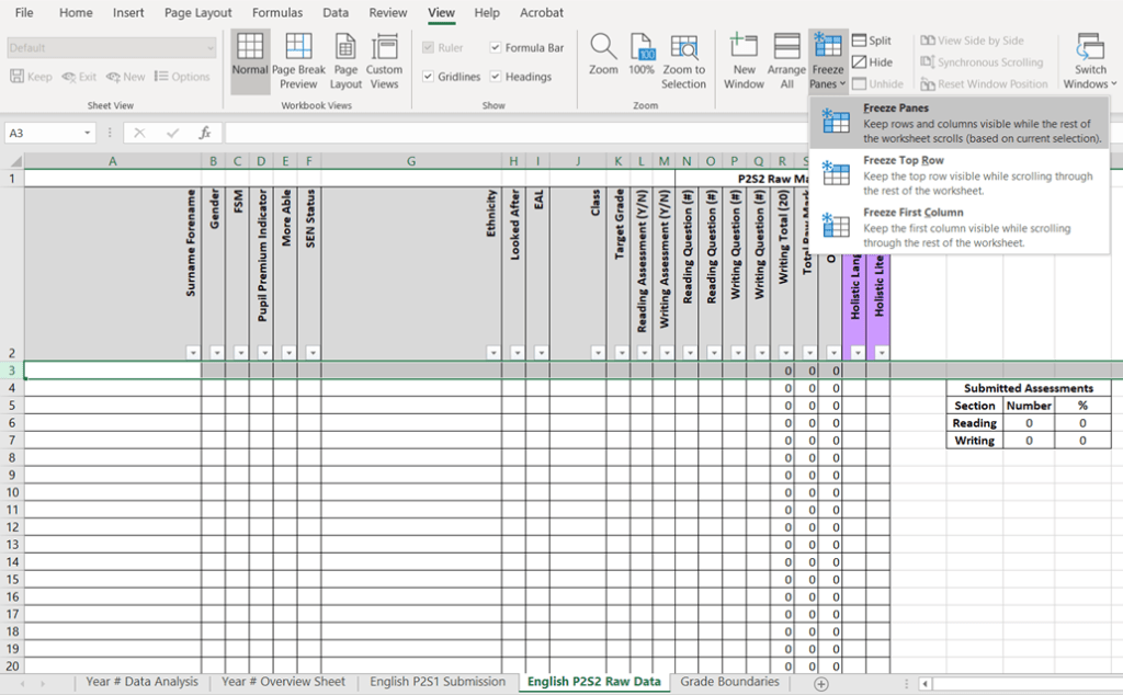
On the top bar, click on ‘View’ then go along to ‘Freeze Panes’. Make sure you select the row or column after the one you want to stay static (in this case the row after the headers). Once selected, simply click ‘Freeze Panes’ and then Ta Da, no more staring at numbers aimlessly trying to make sense of them.

Tip 2

Does everyone else’s trackers look all fancy with a splash of colour here and a dab of colour there? Well, yours can too, in a meaningful way.

Got to love a bit of conditional formatting!

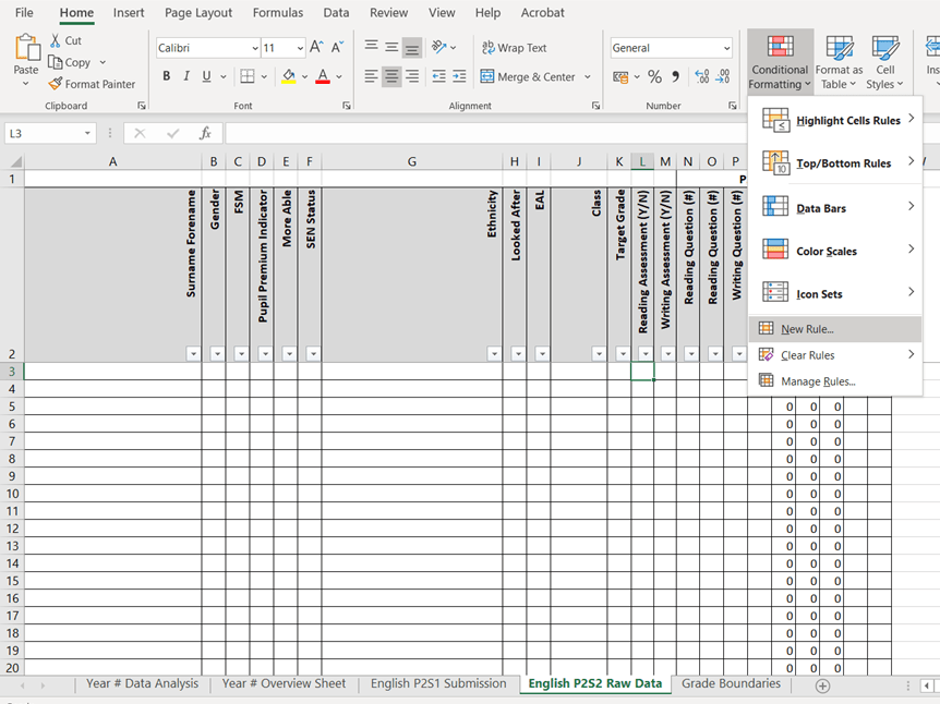
Under the ‘Home’ tab there is the handy option to add a bit of conditional formatting. Now, I like to use this to identify ‘Y/N’ information.

Simply select ‘New Rule’:

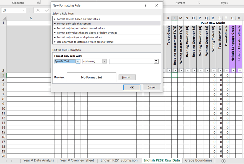
Then ‘Format only cells that contain’ where you need to select ‘Specific Text’ in the first dropdown list. Then put the information you want in the box on the right and select ‘Format…’ where you can change the colour of the cell or the text etc. Once your down, click ‘OK’.

Sometimes, mistakes are made and in our excitement we create a rule we didn’t mean but don’t worry, work through the same process:

‘Home’ Tab > ‘Conditional Formatting’ > ‘Manage Rules’

At which point this little box will pop up and you can delete or edit any of the rules you need to.

If you want to apply that rule to more than one cell, simply click the little square in the right-hand bottom corner of the cell and drag it down to the cell you want. Excel will then copy the rule/s to all the cells you selected.

---

I hope that this helps you out as much as it has helped me out.